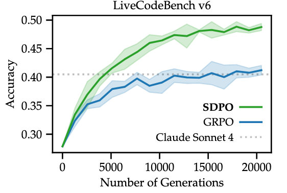
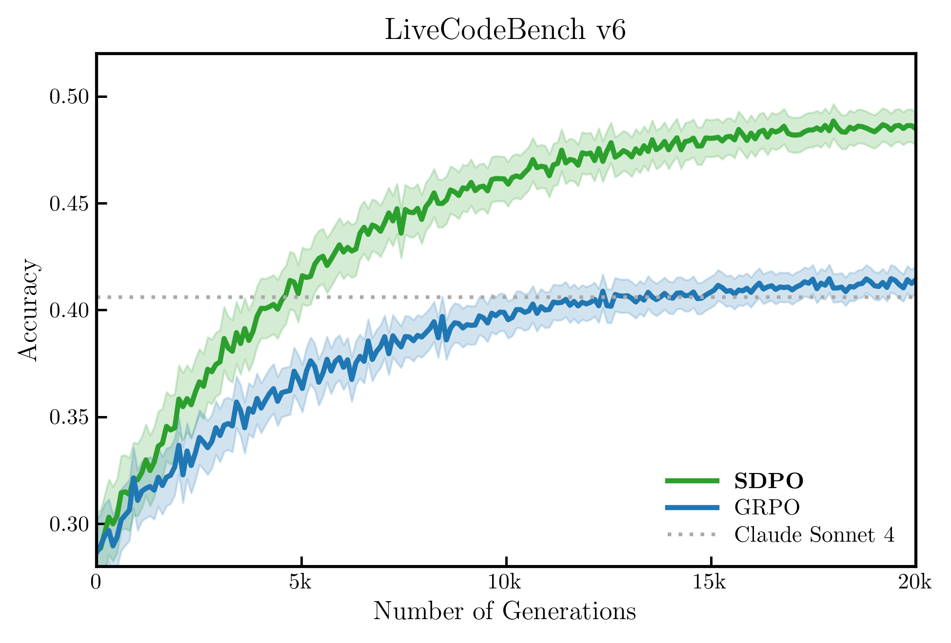
Self-Distillation · LiveCodeBench training curve with confidence band

"""
复现 image2 & image3: Self-distillation 论文折线图
image2: 连续训练曲线 + 置信区间阴影 + 水平参考线
image3: 离散点折线 + 置信区间阴影（模型规模 scaling）
来源：Reinforcement learning via self-distillation
"""

import matplotlib.pyplot as plt
import matplotlib.ticker as ticker
import numpy as np

# ── 预分析结论 ─────────────────────────────────────────────
# 字体：serif，接近 LaTeX Computer Modern，启用 usetex
# 加粗：标题 normal | 图例 SDPO bold | 其他 normal
# Spine：只保留左/下（开口式）
# Grid：无
# 颜色：绿 #3A8B3A (SDPO) | 蓝 #3B6BB5 (GRPO) | 灰 #999999 (base)
# 阴影：主线颜色 alpha=0.15 的半透明填充
plt.rcParams.update({
    'text.usetex': True,
    'font.family': 'serif',
    'font.serif': ['Computer Modern Roman', 'STIX Two Text', 'DejaVu Serif'],
    'axes.unicode_minus': False,
})

C_SDPO  = '#2CA02C'   # matplotlib tab green
C_GRPO  = '#1F77B4'   # matplotlib tab blue
C_BASE  = '#BCBCBC'   # 浅灰，原图 base model

# ══════════════════════════════════════════════════════════
# 图 2：连续训练曲线（LiveCodeBench v6）
# ══════════════════════════════════════════════════════════
np.random.seed(42)

steps = np.linspace(0, 20000, 400)   # 更多点 + EMA 后更平滑

def raw_curve(start, end, steps, noise=0.008):
    t = steps / steps[-1]
    curve = start + (end - start) * (1 - np.exp(-4 * t))
    curve += np.random.normal(0, noise, len(steps)) * (1 - t * 0.7)
    return curve

def ema(arr, alpha=0.96):
    """Exponential moving average — 模拟论文中对 training log 的平滑"""
    out = np.zeros_like(arr)
    out[0] = arr[0]
    for i in range(1, len(arr)):
        out[i] = alpha * out[i - 1] + (1 - alpha) * arr[i]
    return out

# 中心线：先生成有噪声的曲线，再 EMA 平滑（与论文一致）
sdpo_mean = ema(raw_curve(0.285, 0.490, steps, noise=0.006))
sdpo_std  = 0.012 * np.exp(-2 * steps / steps[-1]) + 0.007
grpo_mean = ema(raw_curve(0.285, 0.415, steps, noise=0.006))
grpo_std  = 0.010 * np.exp(-2 * steps / steps[-1]) + 0.006

fig2, ax2 = plt.subplots(figsize=(6.5, 4.4))

ax2.fill_between(steps, sdpo_mean - sdpo_std, sdpo_mean + sdpo_std,
                 color=C_SDPO, alpha=0.20)
ax2.fill_between(steps, grpo_mean - grpo_std, grpo_mean + grpo_std,
                 color=C_GRPO, alpha=0.20)
ax2.plot(steps, sdpo_mean, color=C_SDPO, lw=2.5, label=r'\textbf{SDPO}')
ax2.plot(steps, grpo_mean, color=C_GRPO, lw=2.5, label='GRPO')
# 原图 Claude 参考线为稀疏圆点线，非虚线
ax2.axhline(0.406, color='#AAAAAA', lw=1.8,
            linestyle=(0, (1, 2)), label='Claude Sonnet 4')

ax2.set_xlim(0, 20000)
ax2.set_ylim(0.28, 0.52)
ax2.set_xlabel('Number of Generations', fontsize=13)
ax2.set_ylabel('Accuracy', fontsize=13)
ax2.set_title('LiveCodeBench v6', fontsize=15, pad=7)

ax2.xaxis.set_major_formatter(ticker.FuncFormatter(
    lambda x, _: f'{int(x/1000)}k' if x > 0 else '0'))
ax2.xaxis.set_major_locator(ticker.MultipleLocator(5000))
ax2.yaxis.set_major_locator(ticker.MultipleLocator(0.05))

leg2 = ax2.legend(fontsize=11, loc='lower right',
                  framealpha=0, edgecolor='none',
                  handlelength=2.2, borderaxespad=0.5, labelspacing=0.3)
for text in leg2.get_texts():
    if 'SDPO' in text.get_text():
        text.set_fontweight('bold')

# 四边框 + 向内刻度（与原图一致）
for sp in ax2.spines.values():
    sp.set_visible(True)
    sp.set_linewidth(1.5)
ax2.tick_params(direction='in', length=5, width=1.2, labelsize=11)
ax2.grid(False)

fig2.tight_layout(pad=0.9)
fig2.savefig('line_selfdistill_v6_repro.png',
             dpi=300, facecolor='white')
plt.close(fig2)
print('saved: line_selfdistill_v6_repro.png')

# ══════════════════════════════════════════════════════════
# 图 3：模型 scaling 折线（Model scaling Qwen3）
# ══════════════════════════════════════════════════════════
param_labels = ['0.6', '1.7', '4', '8']
param_x      = [0.6,   1.7,   4,   8]
x_pos        = [0, 1, 2, 3]   # 等间距排列，x 轴用 param_labels

sdpo_pts = [0.215, 0.333, 0.450, 0.490]
grpo_pts = [0.212, 0.295, 0.400, 0.414]
base_pts = [0.095, 0.150, 0.233, 0.284]

sdpo_std3 = [0.005, 0.006, 0.008, 0.006]
grpo_std3 = [0.005, 0.006, 0.007, 0.006]

fig3, ax3 = plt.subplots(figsize=(10, 5))   # 2:1 宽高比，与原图一致

ax3.fill_between(x_pos,
                 [v - s for v, s in zip(sdpo_pts, sdpo_std3)],
                 [v + s for v, s in zip(sdpo_pts, sdpo_std3)],
                 color=C_SDPO, alpha=0.18)
ax3.fill_between(x_pos,
                 [v - s for v, s in zip(grpo_pts, grpo_std3)],
                 [v + s for v, s in zip(grpo_pts, grpo_std3)],
                 color=C_GRPO, alpha=0.18)

MEC = 'black'   # 原图标记点有黑色描边
ax3.plot(x_pos, sdpo_pts, color=C_SDPO, lw=2.5,
         marker='o', ms=7, mfc=C_SDPO,
         markeredgecolor=MEC, markeredgewidth=1.0,
         label=r'\textbf{SDPO}')
ax3.plot(x_pos, grpo_pts, color=C_GRPO, lw=2.5,
         marker='o', ms=7, mfc=C_GRPO,
         markeredgecolor=MEC, markeredgewidth=1.0,
         label='GRPO')
ax3.plot(x_pos, base_pts, color=C_BASE, lw=2.5,   # 与主线同粗
         marker='o', ms=7, mfc=C_BASE,
         markeredgecolor=MEC, markeredgewidth=1.0,
         label='base model')

ax3.set_xticks(x_pos)
ax3.set_xticklabels(param_labels, fontsize=11)
ax3.set_xlim(-0.35, 3.35)
ax3.set_ylim(0.08, 0.51)   # 与原图 0.1~0.5 刻度对齐，留极小顶部空
ax3.set_xlabel('Model parameters (B)', fontsize=13)
ax3.set_ylabel(r'\textit{Accuracy}', fontsize=13)
ax3.set_title('Model scaling (Qwen3)', fontsize=15, pad=7)
ax3.yaxis.set_major_locator(ticker.MultipleLocator(0.1))

# 图例移右下（原图位置）
leg3 = ax3.legend(fontsize=11, loc='lower right',
                  bbox_to_anchor=(0.98, 0.02),
                  framealpha=0, edgecolor='none',
                  handlelength=2.2, borderaxespad=0.5, labelspacing=0.3)
for text in leg3.get_texts():
    if 'SDPO' in text.get_text():
        text.set_fontweight('bold')

# 四边框 + 向内刻度
for sp in ax3.spines.values():
    sp.set_visible(True)
    sp.set_linewidth(1.5)
ax3.tick_params(direction='in', length=5, width=1.2, labelsize=11)
ax3.grid(False)

fig3.tight_layout(pad=0.9)
fig3.savefig('line_selfdistill_scaling_repro.png',
             dpi=300, facecolor='white')
plt.close(fig3)
print('saved: line_selfdistill_scaling_repro.png')