Line Chart · 折线图#test-time-scaling#log-x#confidence-band#reference-line#two-panel
Kronos · Two-panel test-time scaling with std band and dotted baselines
Kronos · 双面板测试时缩放:置信带 + 虚线基线参考
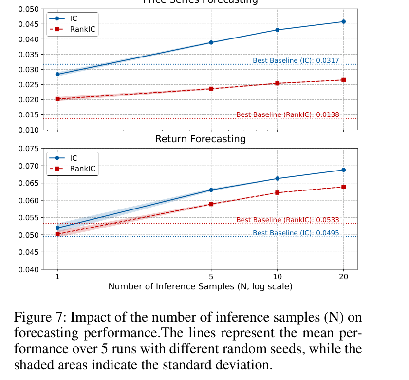
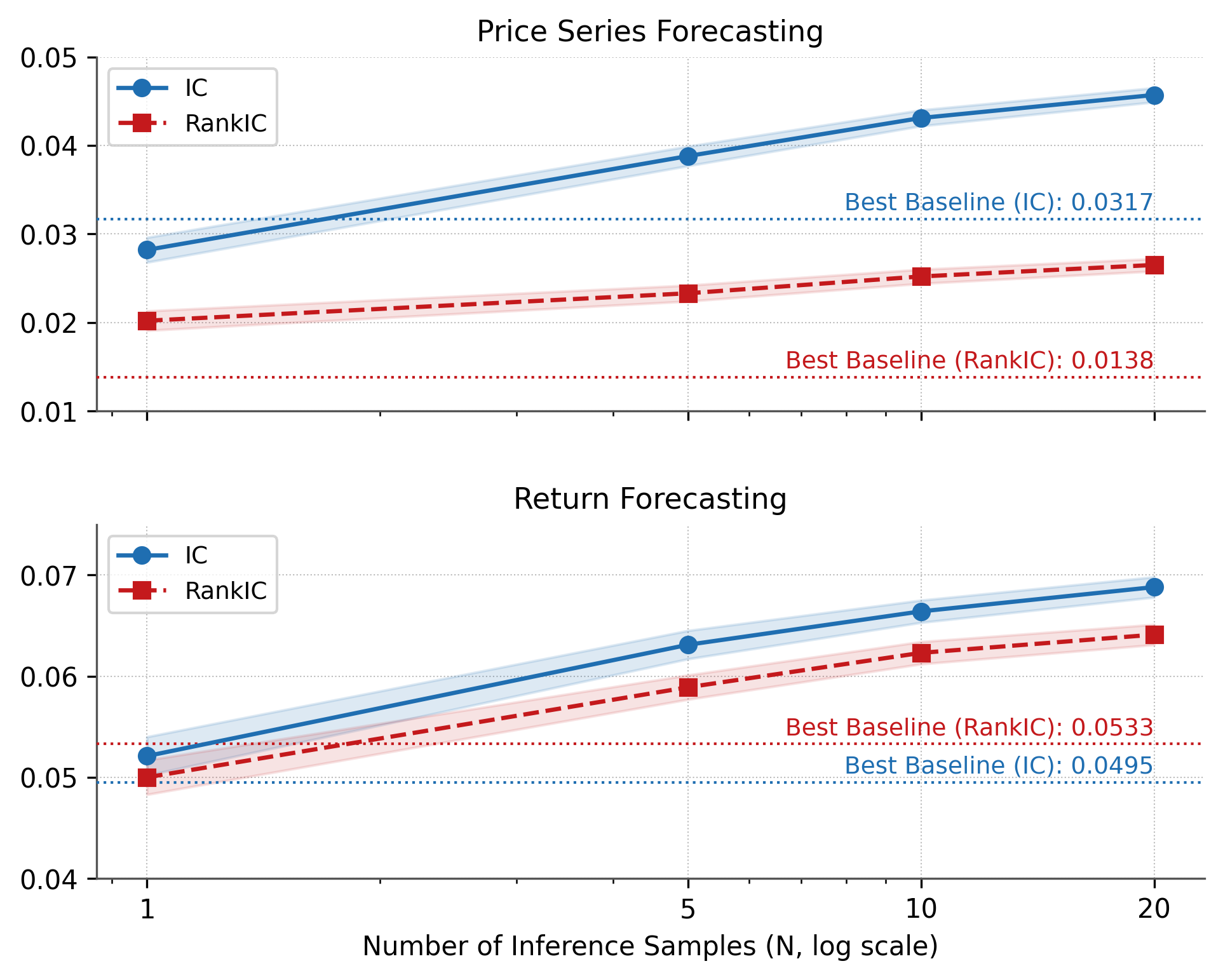
Reproduction of Kronos Figure 7. Two stacked panels (Price Series Forecasting / Return Forecasting) plot IC (solid blue circle) and RankIC (dashed red square) versus the number of stochastic inference samples N on a log x-axis (1, 5, 10, 20). Light shading shows ±1 std over 5 seeds; dotted horizontal lines mark the best non-Kronos baseline IC and RankIC, annotated in matching colour.
Kronos Figure 7 复现。两面板(Price Series Forecasting / Return Forecasting),IC(蓝实线圆点)与 RankIC(红虚线方块)随推理采样数 N(log 轴:1, 5, 10, 20)变化。浅色阴影为 5 个种子的 ±1 std,水平点状参考线标出最优非 Kronos 基线 IC / RankIC,配同色文字标注。
@paper · 来自论文
Kronos: A Foundation Model for the Language of Financial Markets
Kronos:金融市场语言的基础模型
Yu Shi et al. (Tsinghua University) · arXiv 2025
// original from paper · 论文原图
// reproduced via kronos_test_time_scaling.py · 脚本复现download png
kronos_test_time_scaling.py
"""Kronos · Two-panel test-time scaling with confidence band and dotted baselines.

Reproduction of Kronos Figure 7 (Impact of the number of inference samples
N on forecasting performance).
Source: Kronos: A Foundation Model for the Language of Financial Markets,
arXiv:2508.02739.

Two stacked panels (Price Series Forecasting / Return Forecasting) show how
IC (solid blue) and RankIC (dashed red) improve as the number of stochastic
inference samples grows on a log scale. Shaded bands show the standard
deviation across 5 seeds; dotted horizontal lines mark the best non-Kronos
baseline scores.
"""

import matplotlib.pyplot as plt
import numpy as np

plt.rcParams.update({
    "font.family": "sans-serif",
    "font.sans-serif": ["DejaVu Sans", "Arial"],
})

COLOR_IC = "#1F6EB1"
COLOR_RANKIC = "#C4191C"

PRICE_IC_MEAN = np.array([0.0282, 0.0388, 0.0431, 0.0457])
PRICE_IC_STD  = np.array([0.0014, 0.0011, 0.0009, 0.0008])
PRICE_RANKIC_MEAN = np.array([0.0202, 0.0233, 0.0252, 0.0265])
PRICE_RANKIC_STD  = np.array([0.0011, 0.0009, 0.0008, 0.0007])
PRICE_BASE_IC = 0.0317
PRICE_BASE_RANKIC = 0.0138

RETURN_IC_MEAN = np.array([0.0521, 0.0631, 0.0664, 0.0688])
RETURN_IC_STD  = np.array([0.0019, 0.0014, 0.0011, 0.0010])
RETURN_RANKIC_MEAN = np.array([0.0500, 0.0589, 0.0623, 0.0641])
RETURN_RANKIC_STD  = np.array([0.0017, 0.0012, 0.0011, 0.0010])
RETURN_BASE_IC = 0.0495
RETURN_BASE_RANKIC = 0.0533

N = np.array([1, 5, 10, 20])

fig, axes = plt.subplots(2, 1, figsize=(7.5, 5.6), sharex=True)
fig.subplots_adjust(hspace=0.32)

def plot_panel(ax, title, ic_m, ic_s, r_m, r_s, base_ic, base_r,
               ic_baseline_label, r_baseline_label, ylim):
    ax.fill_between(N, ic_m - ic_s, ic_m + ic_s,
                    color=COLOR_IC, alpha=0.15, zorder=2)
    ax.plot(N, ic_m, color=COLOR_IC, marker="o", lw=1.6, ms=6,
            mfc=COLOR_IC, mec=COLOR_IC, label="IC", zorder=4)

    ax.fill_between(N, r_m - r_s, r_m + r_s,
                    color=COLOR_RANKIC, alpha=0.12, zorder=2)
    ax.plot(N, r_m, color=COLOR_RANKIC, marker="s", lw=1.6, ms=6, ls="--",
            mfc=COLOR_RANKIC, mec=COLOR_RANKIC, label="RankIC", zorder=4)

    ax.axhline(base_ic, color=COLOR_IC, lw=1.0, ls=":", zorder=3)
    ax.axhline(base_r,  color=COLOR_RANKIC, lw=1.0, ls=":", zorder=3)
    ax.text(N[-1], base_ic + (ylim[1] - ylim[0]) * 0.012,
            ic_baseline_label, color=COLOR_IC, ha="right",
            va="bottom", fontsize=9)
    ax.text(N[-1], base_r + (ylim[1] - ylim[0]) * 0.012,
            r_baseline_label, color=COLOR_RANKIC, ha="right",
            va="bottom", fontsize=9)

    ax.set_xscale("log")
    ax.set_xticks(N)
    ax.get_xaxis().set_major_formatter(plt.FuncFormatter(lambda v, _: f"{int(v)}"))
    ax.set_title(title, fontsize=11, pad=6)
    ax.set_ylim(*ylim)
    ax.grid(True, ls=":", lw=0.5, color="#bbb", zorder=0)
    ax.set_axisbelow(True)
    ax.legend(loc="upper left", fontsize=9, frameon=True)
    for sp in ("top", "right"):
        ax.spines[sp].set_visible(False)
    for sp in ("left", "bottom"):
        ax.spines[sp].set_color("#555")

plot_panel(axes[0], "Price Series Forecasting",
           PRICE_IC_MEAN, PRICE_IC_STD,
           PRICE_RANKIC_MEAN, PRICE_RANKIC_STD,
           PRICE_BASE_IC, PRICE_BASE_RANKIC,
           f"Best Baseline (IC): {PRICE_BASE_IC:.4f}",
           f"Best Baseline (RankIC): {PRICE_BASE_RANKIC:.4f}",
           ylim=(0.010, 0.050))

plot_panel(axes[1], "Return Forecasting",
           RETURN_IC_MEAN, RETURN_IC_STD,
           RETURN_RANKIC_MEAN, RETURN_RANKIC_STD,
           RETURN_BASE_IC, RETURN_BASE_RANKIC,
           f"Best Baseline (IC): {RETURN_BASE_IC:.4f}",
           f"Best Baseline (RankIC): {RETURN_BASE_RANKIC:.4f}",
           ylim=(0.040, 0.075))

axes[1].set_xlabel("Number of Inference Samples (N, log scale)", fontsize=10)

plt.savefig("kronos_test_time_scaling.png", dpi=300, bbox_inches="tight",
            facecolor="white")
plt.close()
print("saved: kronos_test_time_scaling.png")